基于GANBPSO-SVM的高光谱影像特征选择方法

谢福鼎; 姚娆

doi:10.13249/j.cnki.sgs.2018.06.017

PDF(6056 KB)

地理科学 ›› 2018, Vol. 38 ›› Issue (6) : 972-978. DOI: 10.13249/j.cnki.sgs.2018.06.017

基于GANBPSO-SVM的高光谱影像特征选择方法

作者信息 +

A Feature Selection Strategy for Hyperspectral Images Classification Based on GANBPSO-SVM

Author information +

文章历史 +

摘要

为了在保持对目标检测和分类分析所需信息的同时,降低高光谱影像的维度,提出了一种混合优化策略的特征选择方法。该方法将遗传算法和二进制粒子群优化算法融合成一种新的混合优化策略（GANBPSO）,自动选择最优波段组合,同时优化分类器支持向量机（RBF-SVM）的参数,以提高分类器的分类性能。为了说明所提出方法的有效性,采用了在高光谱分类中广泛使用的Indian Pines（AVIRIS 92AV3C）数据集进行测试。结果表明所提出方法（GANBPSO-SVM）能够自动选择包含最多信息的特征子集以保证分类精度,而不需要预先设置所需要的特征子集数量,本方法与传统方法相比具有更好的分类效果。

Abstract

Rich spectral information from hyperspectral images can aid in the classification and recognition of the ground objects. Currently, hyperspectral images classification has already been applied successfully in various fields. However, the high dimensions of hyperspectral images cause redundancy in information and bring some troubles while classifying precisely ground truth. Hence, this paper proposes a hybrid feature selection strategy based on the Genetic Algorithm and the Novel Binary Particle Swarm Optimization (GANBPSO) to reduce the dimensionality of hyperspectral data while preserving the desired information for target detection and classification analysis. The proposed feature selection approach automatically chooses the most informative features combination. The parameters used in support vector machine (SVM) simultaneously are optimized, aiming at improving the performance of SVM. To show the validity of the proposal, Indian Pines(AVIRIS 92AV3C) data set which is widely used to test the performance of feature selection techniques is chosen to feed the proposed method. The obtained results clearly confirm that the new approach is able to automatically select the most informative features in terms of classification accuracy without requiring the number of desired features to be set a priori by users. Experimental results show that the proposed method can achieve higher classification accuracy than traditional methods.

导出引用

谢福鼎, 姚娆. 基于GANBPSO-SVM的高光谱影像特征选择方法[J]. 地理科学, 2018, 38(6): 972-978 https://doi.org/10.13249/j.cnki.sgs.2018.06.017

Xie Fuding, Yao Rao. A Feature Selection Strategy for Hyperspectral Images Classification Based on GANBPSO-SVM[J]. SCIENTIA GEOGRAPHICA SINICA, 2018, 38(6): 972-978 https://doi.org/10.13249/j.cnki.sgs.2018.06.017

高光谱传感器是利用连续的数百个窄带的电磁波段获取有关地物信息,使原本在宽波段中不可探测的地物在高光谱遥感中得以探测^[1]。与传统遥感影像相比,高光谱遥感影像具有波段连续且数据量大、图谱合一等特点,但存在高维数据的相邻波段冗余度高的问题,这将出现严重的Hughes现象,并导致分类精度低且速度慢^[2]。因此,在更有效地利用高光谱数据的海量信息的基础上,降低特征空间的维数,剔除冗余信息,提高分类的精度和速度已成为高光谱影像分类的重要研究方向之一。

降维技术是解决高光谱影像特征维数高的重要方法。一般地,降维分为特征选择和特征提取^[3]。特征提取是通过映射或变换的方法把原特征转换为较少的新特征,经典的特征提取方法有线性判别分析（LDA）、主成分分析（PCA）、正交子空间投影变换（OSP）及非参数权重特征提取（NWFE）等^[4,5,6]。特征选择是直接从原始波段中选取一定数目最具代表性的波段,不进行变换,因此可以使得地物信息得以保留^[7,8,9]。

在高光谱影像中选择最优波段组合的问题实质上是特征选择并组合优化的过程,其中粒子群算法（PSO）和遗传算法（GA）目前都被广泛应用于高性能优化搜索中,可以快速找到高维空间中的最优解问题^{[8,9,10,11,12,13]}。GA是由Holland等人开发的一种随机搜索算法,模拟Darwin的进化论的自然选择与Mendel的遗传学的生物进化过程的寻优算法^[8]。不同于传统搜索算法,GA从问题的潜在解集即种群开始搜索,所有问题的解即带有特征的个体构成种群。通过选择、交叉、变异等运算生成子代并继续进化,最后收敛于适应度最高的染色体,得到问题的最优解^[9,10]。GA具有广泛寻优能力;PSO具有精度高、收敛快等优点。但是在GA中,如果染色体没被选择来进行配对,那么这个个体就失去了这个染色体所包含的信息,因此GA没有在种群进化的过程中考虑个体自身的发展。而PSO会陷入“早熟”收敛,因为：1）当粒子收敛于全局极值和个体极值时,并不能保证这是局部最优点^[12];2）粒子之间的信息流动很快,容易产生类似的粒子,导致多样性的缺失^[13]。

支持向量机（SVM）在近几年被广泛应用于模式识别领域,因其具有抗噪性能强、对Hughes现象不敏感、学习效率高、结构化风险小等优势^[8]。对于非线性问题,能够利用核技巧将问题映射到高维空间中有效地进行线性分类,在高维模式识别中表现出良好的性能^[14]。采用径向基核函数（RBF）的SVM对高光谱影像进行分类时,惩罚因子C和间隔γ这2个参数能直接影响分类精度,因此,设置合适的SVM参数已成为一个重要的研究方向。通常情况下高光谱影像的特征选择方法都不涉及SVM参数的优化,文献[15]提出了一种基于遗传和标准粒子群结合（HGAPSO）的特征选择的方法,文献[16]提出一种嵌入Hilbert空间的CSVM高光谱影像分类方法,文献[17]提出了一种基于半监督多核SVM的高光谱影像的分类方法,这些方法都没实现特征选择和SVM参数的同步优化。如果SVM参数的值是事先人为设定的,那么在分类过程中就无法自适应的变化以得到更高的分类精度。

基于以上讨论,本文提出了一种GA和PSO相结合的混合优化策略（GANBPSO）,这种混合优化算法由二进制粒子群优化算法（NBPSO）首先进行特征子集的搜索,针对粒子群的“早熟”问题,通过使用GA进行改善^[15]。利用离散型GANBPSO混合优化算法完成特征子集搜索的同时,以连续性PSO对SVM参数进行同步优化。为了说明所提出方法的有效性,本文选取了在高光谱分类中广泛使用的Indian Pines数据集进行实验,结果表明,通过该方法可以获得比传统分类方法更优的分类结果。

1 粒子群优化算法

1.1 经典的粒子群算法

粒子群算法（PSO）是由Kennedy等^[11]开发的一种智能寻优算法,模拟鸟群等群体中个体之间的协作和信息共享来觅食的行为,每个潜在解都看作是D维搜索空间上的一个没有体积的粒子（点）,每个粒子以一定的速度向适应度高的位置飞行,所有的粒子根据自身和同伴的飞行经验在解空间中搜索最优解,粒子i的第d维 (

1 ⩽ d ⩽ D

)的速度用v_id表示,位置用x_id表示,它经历过的最好位置记为p_ibest,所有粒子经历过的最好位置记为p_gbest,对每一代,通过迭代更新速度和位置找寻最优解。首先粒子通过（1）式产生速度^[11]：

v_{id} = w v_{id} + c_{1} r (p_{ibest} - x_{id}) + c_{2} r (p_{gbest} - x_{id})

（1）

再根据（2）式更新位置：

x_{id} = x_{id} + v_{id}

（2）

式中,w为惯性权重,c₁和c₂为不变参数学习因子,r是[0,1]之间的随机值。

1.2 二进制粒子群算法（BPSO）

由于标准PSO用于实值连续空间,Kennedy等人又提出了二进制粒子群算法（BPSO）,BPSO解决了离散组合优化问题,粒子由二进制编码组成,首先通过（1）式产生速度,而用其速度值被转换成二进制位取1的概率,采用（3）式Sigmoid函数将速度映射到区间[0,1]^[18]：

s (v_{id}) = \frac{1}{1 + \exp (- v_{id})}

（3）

而粒子位置更新公式变为（4）：

x_{id} = \{\begin{array}{l} 1 if r \leq s (v_{id}) \\ 0 otherwise \end{array}

（4）

设定v_max作为最大速度值,用于限制位取1或0的概率。

1.3 新的二进制粒子群优化算法

新的二进制粒子群优化算法（NBPSO）的粒子在上一时刻的运动方向和状态决定了下一时刻的更新过程,因此优化效果要优于旧版本的BPSO,粒子的速度更新变为^[19]：

v_{id} = \{\begin{array}{l} v_{id}^{1} if x_{id} = 0 \\ v_{id}^{0} if x_{id} = 1 \end{array}

（5）

式中,

v_{id}^{1}

、

v_{id}^{0}

别表示粒子i的第d维的位置变为1或者0的概率,更新规则为：

v_{id}^{1} = w v_{id}^{1} + d_{id, 1}^{1} + d_{id, 2}^{1}

（6）

v_{id}^{0} = w v_{id}^{0} + d_{id, 1}^{0} + d_{id, 2}^{0}

（7）

式中,

d_{id, 1}^{1}

、

d_{id, 2}^{1}

、

d_{id, 1}^{0}

、

d_{id, 2}^{0}

是根据局部最优值p_ibest、全局最优值p_gbest而变化的临时值,w是惯性权重,

d_{id, 1}^{1}

、

d_{id, 2}^{1}

、

d_{id, 1}^{0}

、

d_{id, 2}^{0}

的更新规则为

if p_{ibest}^{} = 1 Then d_{id, 1}^{1} = c_{1} r_{1} and d_{id, 1}^{0} = - c_{1} r_{1}

if p_{ibest}^{} = 0 Then d_{id, 1}^{0} = c_{1} r_{1} and d_{id, 1}^{1} = - c_{1} r

if p_{gbest}^{} = 1 Then d_{id, 2}^{1} = c_{2} r_{2} and d_{id, 2}^{0} = - c_{2} r

if p_{gbest}^{} = 0 Then d_{id, 2}^{0} = c_{2} r_{2} and d_{id, 2}^{1} = - c_{2} r_{2}

式中,r₁、r₂是[0,1]之间的随机值,c₁和c₂是不变参数学习因子。当p_ibest或p_gbest为0时,

d_{id, 1}^{0}

、

d_{id, 2}^{0}

为正值,

v_{id}^{0}

增加;

d_{id, 1}^{1}

、

d_{id, 2}^{1}

为负值,

v_{id}^{1}

减小。反之,当p_ibest或p_gbest为1时,

v_{id}^{0}

减小,

v_{id}^{1}

增加。通过这种方式,在粒子更新的过程中考虑了前一时刻的状态,粒子某一位变为1或0的方向也能保持下去,因此取得了良好的优化效果。粒子位置的更新公式为：

x_{id} = \{\begin{array}{l} {\overset{̅}{x}}_{id} if r_{id} \leq {v^{'}}_{id} \\ x_{id} if r_{id} > {v^{'}}_{id} \end{array}

（8）

式中,

{\overset{̅}{x}}_{id}

表示x_id在二进制下的取反,r_id是在[0,1]区间的随机数。

2 基于GANBPSO-SVM的特征选择与分类

混合优化算法结合了GA和PSO算法的优点,在PSO中引入GA中的选择、交叉和变异策略,避免陷入局部最优,得到适应度更高的下一代优秀种群。混合优化算法步骤如下：

步骤1：初始化。包括种群规模N,随机给出初始粒子位置和速度;惯性权值w及最大迭代次数。

步骤2：编码。编码后的粒子包括特征掩码和SVM参数2个部分,每个粒子共有D+2维,前D维表示特征掩码,后2维是SVM的参数C和γ（见图1）。其中特征掩码部分是把每个特征转换为一维离散二进制串,每个粒子代表一个不同的特征子集,如果第i位为1,则第i个特征就被选中,否则被隐藏,粒子的长度等于所有特征子集的数量,即原始波段数目。编码上的数值对应当前的位置信息,通过迭代更新速度和位置找寻最优解。特征掩码将每个特征进行二进制转换因此是由0、1组成,用离散型的GANBPSO算法进行特征选择;而SVM参数并不进行二进制转换,用实数表示,更新方式采用连续型的PSO算法进行寻优。

图1 粒子编码

Fig.1 Particle’s encoding

Full size|PPT slide

步骤3：适应度评价。高光谱影像特征选择的目的是在保证分类精度的前提下,选择尽可能少的特征子集,因此适应度函数从分类精度和特征子集两方面考虑,采用权重的方法作为适应度函数：

fitness = a \cdot OA + b \cdot (1 - N_{0} / N)

（9）

式中,OA表示当前特征子集的总体分类精度;a+b=1,且a,b>0;N₀表示当前特征子集的个数,N为特征总个数,即粒子个数。

步骤4：粒子更新。

1）首先采用NBPSO算法,根据式（5）和式（8）对粒子的特征掩码部分的速度和位置进行更新。再根据式（2）对粒子的SVM参数部分进行更新。

2）计算每个粒子的适应度,按照适应度从大到小排序,选择适应度高的前N/2优选粒子直接进入下一代,后N/2粒子进行GA的交叉和变异操作。

3）将这2次更新后分别得到的N/2粒子重新组成下一代种群。

步骤5：收敛判断。终止条件为连续5次计算出的适应度值的上下浮动小于给定的阈值ε;或达到最大迭代次数,选取种群中适应度最高的粒子作为最优的特征子集。否则转到步骤4重新执行。

3 实验及结果分析

本文采用AVIRIS传感器获取的美国印第安纳州测试地（Indian Pines）的高光谱影像数据^[20]进行了试验,该数据共220个波段,空间分辨率为20 m,图像大小为145×145,波长覆盖范围0.4~2.5 μm。除去水汽和噪声吸收较为明显的波段,剩下的200个波段用于特征子集的选择和分类研究。该数据包括16个地物类型,每个类别随机选取10％的标记样本作为训练集,剩下的作为测试集（见表1）。图2分别为50、17、27波段合成的伪彩色图和测试影像的参考图及包含的各类地物像素数^[21]（其中白色部分为背景,在分类的过程中剔除）。

表1 训练集和测试集

Table 1 Number of training and test samples

类别号	类别名称	训练集	测试集
1	苜蓿	5	41
2	免耕玉米	143	1285
3	少耕玉米	83	747
4	玉米地	24	213
5	牧场	49	434
6	树	73	657
7	收割牧草	3	25
8	干草匀堆料	48	430
9	燕麦	2	18
10	免耕大豆	98	874
11	少耕大豆	246	2209
12	净耕大豆	60	533
13	小麦	21	184
14	木材	127	1138
15	建筑-草地-树木-机器	39	347
16	石钢塔	10	83
	共计	1031	9218

图2 高光谱 数据集（a）和相应的参考数据（b）
图例括号中数字为像素点个数。

Fig.2 Hyperspectral datasets (a) and the corresponding reference data (b)

Full size|PPT slide

3.1 实验参数

实验中群体规模取40,粒子的初始速度为0,学习因子c₁=c₂=2,惯性权重w由1到0.5线性减少,解空间维数为202,其中后2维表示SVM参数C和γ,取值范围分别为C∈[1,1000]和γ∈[0,20],迭代次数为300次,阈值ε=0.05。

3.2 精度评价

表征分类结果的指标有很多,其中最常用的是利用混淆矩阵、总体分类精度及Kappa系数^[22]。

3.2.1 总体分类精度

总体分类精度指被正确分类的类别像元数与总像元数的比值,计算公式如下^[22]：

OA = \frac{\overset{r}{\sum_{i = 1}} x_{ii}}{N}

（10）

式中,N是总像元数,r是混淆矩阵的行数即类别数,x_ii是i行i列（混淆矩阵对角线）的值即被正确分类的像元数。

3.2.2 Kappa系数

Kappa系数代表分类与完全随机分类产生错误减少的比例,公式如下^[22]：

KC = \frac{N \overset{r}{\sum_{i = 1}} x_{ii} - \sum^{} (x_{i +} \times x_{+ i})}{N^{2} - \sum^{} (x_{i +} \times x_{+ i})}

（11）

式中,x_i+和x_+i分别代表各行与各列之和。

KC值与分类效果的对应关系如表2所示^[22]。

表2 KC统计值与分类效果对应关系

Table 2 Classification quality associated to the Kappa statistics value

KC	分类效果
<0	较差
0~0.2	差
0.2~0.4	正常
0.4~0.6	好
0.6~0.8	较好
0.8~1.0	非常好

3.3 实验评价

为了验证本文算法的有效性,本文进行了多组实验。首先,为了验证SVM分类器的可靠性和优化SVM参数的有效性,进行了多组不同分类器的对比实验。然后采用不同特征选择算法优选出的特征子集进行分类比较,以验证GANBPSO的有效性。

3.3.1 基于不同分类器的对比分类实验

在原始200个波段下进行高光谱影像分类,将SVM与极限学习机（ELM）和K最近邻（KNN）分类方法进行比较,以验证选择RBF-SVM作为分类器的合理性,对优化参数前后的分类结果进行比较,以验证参数优化上的优势,训练数据和测试数据集如表2所示。从表3可以看出,SVM分类方法取C=100,γ=2时得到的分类精度比ELM和KNN分别高出7.95%和5.12%,显然以SVM作为分类器在分类结果上有一定的优势。同时,惩罚因子C和间隔γ采用不同的数值,分类精度也不同,说明C和γ直接影响到了分类的精度,因此优化SVM的2个参数是有意义的。

表3 不同分类器200个波段下的分类精度

Table 3 Classification accuracy by different classifiers in the original hyperspectral image

分类方法	参数范围	OA(%)	KC
ELM	N∈[5,50]	71.09	0.6873
KNN	K∈[1,15]	73.92	0.6920
SVM	C=100,γ=2	79.04	0.7611
	C=120,γ=2	78.74	0.7588
	C=200,γ=6	81.80	0.7930

表4给出了优化SVM参数前后的分类试验结果对比结果。采用GANBPSO进行特征选择后,最终得到的适应度最大的粒子中,长度为200的特征子集二进制串中位长为1的个数是44,即得到了44个特征子集组合,最后2维所对应的最优参数组合中C和γ分别取241.616 9和8.196 1。优化后,波段数从200降到44,大大降低了高光谱影像的维度。并且在选择特征子集的同时,SVM的参数C和γ也得到了优化,相对于事先指定参数值的SVM的分类,精度也从81.80%提升到85.56%。显然,经过GANBPSO方法优选子集和优化SVM参数后,不仅能剔除冗余子集得到优选特征子集组合,还能优化SVM分类器的性能,大幅度的提升了分类精度。

表4 特征选择和SVM参数优化前后的分类精度

Table 4 Classification accuracy of SVM parameters optimization

分类方法	波段数	参数	OA(%)	KC
SVM	200	C=200,γ=6	81.80	0.7930
GANBPSO-SVM	44	C=241.6169,γ=8.1961	85.56	0.8323

3.3.2 基于不同特征选择算法的对比分类实验

PSO和GAPSO都是常用的寻优算法,在高光谱影像的特征选择中得到了广泛的应用。为了验证本文特征选择方法相比传统特征选择方法具有更好的效果,本实验分别采用PSO^[15]、HGAPSO^[15]和本文提出的GANBPSO三种不同的特征选择方法（3种方法均为各类随机选取10％的训练样本）基于SVM进行分类,将3次优选出来的特征子集的分类精度进行比较,训练集和测试集如表1所示。图3中的(b) (c) (d)分别显示了PSO-SVM^[15]、HGAPSO-SVM^[15]和GANBPSO-SVM的可视化分类结果。从表5可以轻易看出,对200个原始波段进行特征选择后分类结果相对于原始波段均有不同程度的提高,而本文提出的GANBPSO算法的精度优于其他2个算法,说明GANBPSO算法能得到更优的特征子集组合,并在优化SVM分类器参数的同时,提高了分类器的性能,达到了较好的分类精度（表5）。

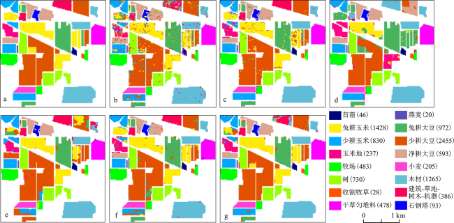
图3 分类结果对比
图例括号中数字为像素点个数。
a.参考数据; b. PSO- SVM分类结果（10%训练样本）; c. HGAPSO- SVM分类结果（10%训练样本）; d. GANBPSO-SVM（10%训练样本）分类结果; e. GANBPSO-SVM（20%训练样本）分类结果; f. GANBPSO-SVM（50%训练样本）分类结果; g.GANBPSO-SVM（80%训练样本）分类结果

Fig.3 Comparison of the classification results

Full size|PPT slide

表5 基于SVM的不同特征选择方法的分类精度

Table 5 classification accuracy by different feature selection algorithms based on SVM

分类方法	OA（%）	KC
PSO-SVM^[15]	74.69	0.7289
HGAPSO-SVM^[15]	76.08	0.7495
GANBPSO-SVM	85.56	0.8323

3.3.3 不同比例训练样本数的分类结果

采用本文提出的GANBPSO-SVM方法,分别选择10%、20%、50%、80%的样本数据作为训练数据集,对不同比例训练样本进行分类,迭代次数设定为300次,分类精度如表6,分类效果如图3所示。如表中所示,分类精度随着训练样本比例的增高而增高,说明训练样本比例越高,影像的分类精度越高,越能体现目标地物的特征。

表6 基于GANBPSO-SVM的不同比例训练样本的分类结果

Table 6 Classification accuracy based on GANBPSO-SVM under different proportions of the training samples

类别	训练样本比例（%）
类别	10	20	50	80
OA（%）	85.56	87.99	91.04	94.61
KC	0.8323	0.8623	0.8946	0.9384

4 结语

针对PSO在特征选择时容易“早熟”的问题,本文提出了一种基于遗传算法和二进制粒子群优化算法相结合的混合优化策略。所提出的方法不仅得到了最优特征（波段）子集,降低了特征的维数,而且优化了SVM算法中的参数,克服了分类结果随参数变化的缺点。实验结果表明,本文得到的分类结果优于其它利用PSO和SVM组合算法得到结果。本文在利用SVM分类的时候仅考虑了谱信息,没有充分利用到高光谱影像的其它信息如空间特征、形状特征及纹理特征等,如何实现“空-谱”合一,这是一个值得进一步研究的问题。

参考文献

列表( 原文顺序 | 文献年度倒序 | 文中引用次数倒序 ) 可视化分析

[1]	Yuen P W, Richardson M.An introduction to hyperspectral imaging and its application for security, surveillance and target acquisition[J]. Journal of Photographic Science, 2013, 58(5):241-253. 本文引用 [1]

[2]

Bruzzone

, Serpico S

.A technique for feature selection in multiclass problems[J]. International Journal of Remote Sensing, 2000, 21(3):549-563.

One of the main phases in the development of a system for the classification of remote sensing images is the definition of an effective set of features to be given as input to the classifier. In particular, it is often useful to reduce the number of features available, while saving the possibility to discriminate among the different land-cover classes to be recognized. This paper addresses this topic with reference to applications that involve more than two land-cover classes (multiclass problems). Several criteria proposed in the remote sensing literature are considered and compared with one another and with the criterion presented by the authors. Such a criterion, unlike those usually adopted for multiclass problems, is related to an upper bound to the error probability of the Bayes classifier. As the objective of feature selection is generally to identify a reduced set of features that minimize the errors of the classifier, the aforementioned property is very important because it allows one to select features by taking into account their effects on classification errors. Experiments on two remote sensing datasets are described and discussed. These experiments confirm the effectiveness of the proposed criterion, which performs slightly better than all the others considered in the paper. In addition, the results obtained provide useful information about the behaviour of different classical criteria when applied in multiclass cases.

https://doi.org/10.1080/014311600210740

http://www.tandfonline.com/doi/abs/10.1080/014311600210740

本文引用 [1]

[3]	边肇祺, 张学工. 模式识别第2版[M]. 北京: 清华大学出版社, 2000:176-210. [Bian Zhaoqi, Zhang Xuegong.Pattern recognition. Beijing: Tsinghua University Press, 2000:176-210.] 本文引用 [1]

[4]	Nixon M, Aguado A S.Feature Extraction and Image Processing[J]. Academic Press, 2012, 44(4):595-599. 本文引用 [1]

[5]

赵泉华, 王玉, 李玉. 利用SAR影像区域分割方法提取海洋暗斑特征[J]. 地理科学, 2016, 36(1):121-127.

在SAR强度影像中,包括海洋溢油在内的许多海洋现象呈现为暗斑。为从诸多暗斑中辨识海洋溢油,需要在SAR影像中提取暗斑的几何和统计分布特征,以此作为进一步分类(辨识)海洋溢油的依据,将基于几何划分技术的区域分割方法应用于SAR影像暗斑特征提取。首先建立高分辨率SAR影像暗斑或然率模型,然后利用最大化期望值和M-H算法实现其几何及统计分布特征参数提取。实验结果表明,该方法不仅可以精准提取暗斑的几何形状,同时还能有效估计其统计分布参数。

https://doi.org/10.1329/j.cnki.sgs.2016.01.015

http://www.cqvip.com/QK/95809X/201601/667837285.html

[Zhao

Quanhua

, Wang

, Li

.Feature extraction of Dark Spot based on the SAR image segmentation. Scientia Geographica Sinica, 2016, 36(1):121-127.]

本文引用 [1]

[6]	Ghamisi P, Benediktsson, J A Cavallaro G et al. Automatic framework for spectral-spatial classification based on supervised feature extraction and morphological attribute profiles[J]. IEEE Journal of Selected Topics in Applied Earth Observations & Remote Sensing, 2014, 7(6):2147-2160 本文引用 [1]

[7]

王芳, 卓莉, 黎夏,等. 基于高光谱特征选择和RBFNN的城市植被胁迫程度监测[J]. 地理科学, 2008, 28(1):77-82.

以Hyperion星载高光谱数据为例,基于指数提取-特征选择-分类识别-模式分析的思路,分析广州市的城市植被胁迫状况。提取与胁迫相关的高光谱植被指数,对其进行相关分析,滤除相关性很高的植被指数,利用选取的特征应用RBF(径向基函数)神经网络对城市的植被胁迫程度进行分类,对广州市受胁迫植被的空间分布及其原因进行分析。研究表明:运用特征选取和RBF神经网络可以较好的区分城市植被受胁迫的程度;城市植被受胁迫的程度与城市交通污染、人为干扰相关性比较大;受胁迫植被的强度分布呈现从城市中心向外的梯度变化,在大块绿地外围呈环状分布。

[Wang

Fang

, Zhuo

, Li

Xia

et al. Urban vegetation stress level monitoring based on hyperspectral feature selection and RBF neural Network. Scientia Geographica Sinica,2008,28(1):77-82.]

本文引用 [1]

[8]

Shijin

, Wu

Hao

,Wan

Dingsheng

et al. An effective feature selection method for hyperspectral image classification based on genetic algorithm and support vector machine[J]. Knowledge-Based Systems, 2011, 24(1):40-48.

https://doi.org/10.1016/j.knosys.2010.07.003

http://linkinghub.elsevier.com/retrieve/pii/S0950705110001097

本文引用 [4]

[9]

Pal

.Hybrid genetic algorithm for feature selection with hyperspectral data[J]. Remote Sensing Letters, 2013, 4(7):619-628.

This letter evaluates the performance of a wrapper–filter genetic algorithm (GA) for feature selection using Digital Airborne Imaging Spectrometer hyperspectral data set. Classification accuracy by k-nearest neighbour (k-NN) and support vector machine (SVM) were used as fitness function with four filter algorithms. Results of wrapper–filter GA-based feature selection approach were compared with a steady-state GA-based approach in terms of number of selected features and the accuracy with selected feature. Result indicates the unsuitability of SVM as wrapper due to large computational cost in comparison to k-NN. Choice of filter algorithm seems to be having no significant effect on classification accuracy obtained using selected features. Comparison in terms of number of selected features and the accuracy with selected features suggests comparable performance by both wrapper–filter and steady-state GAs for the used data set.

https://doi.org/10.1080/2150704X.2013.777485

http://www.tandfonline.com/doi/abs/10.1080/2150704X.2013.777485

本文引用 [3]

[10]

Cui

Minshan

, Prasad

, Li

Wei

et al. Locality preserving genetic algorithms for spatial-spectral hyperspectral image classification[J]. IEEE Journal of Selected Topics in Applied Earth Observations & Remote Sensing, 2013, 6(3):1688-1697.

Recent developments in remote sensing technologies have made hyperspectral imagery (HSI) readily available to detect and classify objects on the earth using pattern recognition techniques. Hyperspectral signatures are composed of densely sampled reflectance values over a wide range of the spectrum. Although most of the traditional approaches for HSI analysis entail per-pixel spectral classification, spatial-spectral exploitation of HSI has the potential to further improve the classification performance-particularly when there is unique class-specific textural information in the scene. Since the dimensionality of such remotely sensed imagery is often very large, especially in spatial-spectral feature domain, a large amount of training data is required to accurately model the classifier. In this paper, we propose a robust dimensionality reduction approach that effectively addresses this problem for hyperspectral imagery (HSI) analysis using spectral and spatial features. In particular, we propose a new dimensionality reduction algorithm, GA-LFDA where a Genetic Algorithm (GA) based feature selection and Local-Fisher's Discriminant Analysis (LFDA) based feature projection are performed in a raw spectral-spatial feature space for effective dimensionality reduction. This is followed by a parametric Gaussian mixture model classifier. Classification results with experimental data show that our proposed method outperforms traditional dimensionality reduction and classification algorithms in challenging small training sample size and mixed pixel conditions.

https://doi.org/10.1109/JSTARS.2013.2257696

http://ieeexplore.ieee.org/document/6516604/

本文引用 [2]

[11]

Yang

, Du

Qian

, Chen

Genshe

.Particle swarm optimization-based hyperspectral dimensionality reduction for urban land cover classification[J]. IEEE Dournal of Selected Topics in Applied Earth Observations and Remote Sensing,2012,5(2):544-554.

https://doi.org/10.1109/JSTARS.2012.2185822

http://ieeexplore.ieee.org/document/6162969/

本文引用 [3]

[12]

Frans V D

, Engelbrecht A

. A cooperative approach to particle swarm optimization[J]. IEEE Transactions on Evolutionary Computation, 2004, 8(3):225-239.

The particle swarm optimizer (PSO) is a stochastic, population-based optimization technique that can be applied to a wide range of problems, including neural network training. This paper presents a variation on the traditional PSO algorithm, called the cooperative particle swarm optimizer, or CPSO, employing cooperative behavior to significantly improve the performance of the original algorithm. This is achieved by using multiple swarms to optimize different components of the solution vector cooperatively. Application of the new PSO algorithm on several benchmark optimization problems shows a marked improvement in performance over the traditional PSO.

https://doi.org/10.1109/TEVC.2004.826069

http://ieeexplore.ieee.org/document/1304845/

本文引用 [2]

[13]

Premalatha

, Natarajan A

.Hybrid PSO and GA for Global Maximization[J]. Icsrs Int.j.open Problems Compt.math, 2009, 2(4):597-608.

Summary: This paper present the hybrid approaches of Particle Swarm Optimization (PSO) with Genetic Algorithm (GA). PSO and GA are population based heuristic search technique which can be used to solve the optimization problems modeled on the concept of Evolutionary Approach. In standard PSO, the non-oscillatory route can quickly cause a particle to stagnate and also it may prematurely converge on suboptimal solutions that are not even guaranteed to be local optimum. In this paper the modification strategies are proposed in PSO using GA. Experiment results are examined with benchmark functions and results show that the proposed hybrid models outperform the standard PSO.

http://www.ams.org/mathscinet-getitem?mr=2570009

本文引用 [2]

[14]

Mingmin

, Bruzzone

.Semisupervised classification of hyperspectral images by SVMs optimized in the Primal[J]. IEEE Transactions on Geoscience and Remote Sensing, 2007, 45(6): 1870-1880.

This paper addresses classification of hyperspectral remote sensing images with kernel-based methods defined in the framework of semisupervised support vector machines (S3VMs). In particular, we analyzed the critical problem of the nonconvexity of the cost function associated with the learning phase of S3VMs by considering different (S3VMs) techniques that solve optimization directly in the primal formulation of the objective function. As the nonconvex cost function can be characterized by many local minima, different optimization techniques may lead to different classification results. Here, we present two implementations, which are based on different rationales and optimization methods. The presented techniques are compared with S3VMs implemented in the dual formulation in the context of classification of real hyperspectral remote sensing images. Experimental results point out the effectiveness of the techniques based on the optimization of the primal formulation, which provided higher accuracy and better generalization ability than the S3VMs optimized in the dual formulation

https://doi.org/10.1109/TGRS.2007.894550

http://ieeexplore.ieee.org/document/4215036/

本文引用 [1]

[15]

Ghamisi

, Benediktsson J

.Feature selection based on hybridization of genetic algorithm and particle swarm optimization[J]. IEEE Geoscience & Remote Sensing Letters, 2015, 12(2):309-313.

A new feature selection approach that is based on the integration of a genetic algorithm and particle swarm optimization is proposed. The overall accuracy of a support vector machine classifier on validation samples is used as a fitness value. The new approach is carried out on the well-known Indian Pines hyperspectral data set. Results confirm that the new approach is able to automatically select the most informative features in terms of classification accuracy within an acceptable CPU processing time without requiring the number of desired features to be set a priori by users. Furthermore, the usefulness of the proposed method is also tested for road detection. Results confirm that the proposed method is capable of discriminating between road and background pixels and performs better than the other approaches used for comparison in terms of performance metrics.

https://doi.org/10.1109/LGRS.2014.2337320

http://ieeexplore.ieee.org/document/6866865/

本文引用 [8]

[16]

Gurram

, Kwon

.Contextual SVM Using Hilbert Space Embedding for Hyperspectral Classification[J]. IEEE Geoscience & Remote Sensing Letters, 2013, 10(5):1031-1035.

In this letter, a kernel-based contextual classification approach built on the principle of a newly introduced mapping technique, called Hilbert space embedding, is proposed. The proposed technique, called contextual support vector machine (SVM), is aimed at jointly exploiting both local spectral and spatial information in a reproducing kernel Hilbert space (RKHS) by collectively embedding a set of spectral signatures within a confined local region into a single point in the RKHS that can uniquely represent the corresponding local hyperspectral pixels. Embedding is conducted by calculating the weighted empirical mean of the mapped points in the RKHS to exploit the similarities and variations in the local spectral and spatial information. The weights are adaptively estimated based on the distance between the mapped point in consideration and its neighbors in the RKHS. An SVM separating hyperplane is built to maximize the margin between classes formed by weighted empirical means. The proposed technique showed significant improvement over the composite kernel-based SVM on several hyperspectral images.

https://doi.org/10.1109/LGRS.2012.2227934

http://ieeexplore.ieee.org/document/6458981/

本文引用 [1]

[17]

Sun

Zhuo

, Wang

Cheng

, Wang

Hanyun

et al. Learn multiple-kernel SVMs for domain adaptation in hyperspectral data[J]. IEEE Geoscience & Remote Sensing Letters, 2013, 10(5):1224-1228.

This letter presents a novel semisupervised method for addressing a domain adaptation problem in the classification of hyperspectral data. To overcome the influence of distribution bias between the source and target domains, we introduce the domain transfer multiple-kernel learning to simultaneously minimize the maximum mean discrepancy criterion and the structural risk functional of support vector machines. Then, the pairwise binary classifiers are merged as the multiclass classifier for solving the classification problem in hyperspectral data. Both bias and nonbias sampling strategies are introduced to evaluate the robustness of the proposed method against the spectral distribution bias. The results obtained from real data sets show that the proposed method can achieve higher classification accuracy even with cross-domain distribution bias and provide robust solutions with different labeled and unlabeled data sizes.

https://doi.org/10.1109/LGRS.2012.2236818

http://ieeexplore.ieee.org/document/6470638/

本文引用 [1]

[18]	Kennedy J, Eberhart R C.A discrete binary version of the particle swarm algorithm[C]//IEEE. IEEE international conference on systems, Man, and Cybernetics, 1997. Computational Cybernetics and Simulation, 1997:4104-4108. 本文引用 [1]

[19]	Khanesar M A, Teshnehlab M, Shoorehdeli M A.Novel binary particle swarm optimization[M]//Aleksandar Lazinica. Particle swarm optimization in tech, 2007:1-6. 本文引用 [1]

[20]	Landgrebe D A.Indiana’s Pines Dataset[EB/ OL]. 2009-08-10.tp. ftp://ftp. ecn. purdue. edu/ biehl/ MultiSpec/ 92AV3C(original files 本文引用 [1]

[21]	Landgrebe D A.ftp:MultiSpec/ ThyFiles Indiana’s Pines Dataset[EB/OL].2009-08-10. //ftp. ecn. purdue. edu/ biehl/ PCzip (ground truth). 本文引用 [1]

[22]	Landis J R, Koch G G.An application of hierarchical kappa-type statistics in the assessment of majority agreement among multiple observers.[J]. Biometrics, 1977, 33(2):363-74. https://doi.org/10.2307/2529786 https://www.jstor.org/stable/2529786?origin=crossref 本文引用 [4]

脚注

The authors have declared that no competing interests exist.

基金

国家自然科学基金项目（41771178,61772252）、广东省数学与交叉科学普通高校重点实验室开放项目资助

PDF(6056 KB)

可视化

2713

Accesses

Citation

Detail

段落导航

摘要
Abstract
关键词
Key words
引用本文
1 粒子群优化算法
1.1 经典的粒子群算法
1.2 二进制粒子群算法（BPSO）
1.3 新的二进制粒子群优化算法
2 基于GANBPSO-SVM的特征选择与分类
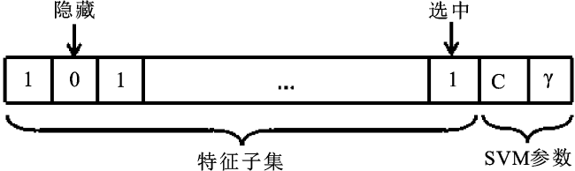
图1 粒子编码
3 实验及结果分析
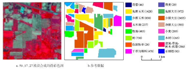
表1 训练集和测试集
图2 高光谱数据集（a）和相应的参考数据（b）图例括号中数字为像素点个数。
3.1 实验参数
3.2 精度评价
表2 KC统计值与分类效果对应关系
3.3 实验评价
表3 不同分类器200个波段下的分类精度
表4 特征选择和SVM参数优化前后的分类精度
图3 分类结果对比图例括号中数字为像素点个数。a.参考数据; b. PSO- SVM分类结果（10%训练样本）; c. HGAPSO- SVM分类结果（10%训练样本）; d. GANBPSO-SVM（10%训练样本）分类结果; e. GANBPSO-SVM（20%训练样本）分类结果; f. GANBPSO-SVM（50%训练样本）分类结果; g.GANBPSO-SVM（80%训练样本）分类结果
表5 基于SVM的不同特征选择方法的分类精度
表6 基于GANBPSO-SVM的不同比例训练样本的分类结果
4 结语
参考文献
脚注
基金

收稿日期	修回日期	出版日期
2017-06-12	2017-08-04	2018-06-20
发布日期
2018-06-20

选择文件类型/文献管理软件名称

选择包含的内容

摘要

Abstract

关键词

Key words

引用本文

1 粒子群优化算法

1.1 经典的粒子群算法

1.2 二进制粒子群算法（BPSO）

1.3 新的二进制粒子群优化算法

2 基于GANBPSO-SVM的特征选择与分类

图1 粒子编码

3 实验及结果分析

表1 训练集和测试集

图2 高光谱 数据集（a）和相应的参考数据（b）
图例括号中数字为像素点个数。

3.1 实验参数

3.2 精度评价

表2 KC统计值与分类效果对应关系

3.3 实验评价

表3 不同分类器200个波段下的分类精度

表4 特征选择和SVM参数优化前后的分类精度

表5 基于SVM的不同特征选择方法的分类精度

表6 基于GANBPSO-SVM的不同比例训练样本的分类结果

4 结语

{{custom_sec.title}}

{{custom_sec.title}}

参考文献

脚注

{{custom_fnGroup.title_cn}}

脚注

基金

模态框（Modal）标题

选择文件类型/文献管理软件名称

选择包含的内容

摘要

Abstract

关键词

Key words

引用本文

1 粒子群优化算法

1.1 经典的粒子群算法

1.2 二进制粒子群算法（BPSO）

1.3 新的二进制粒子群优化算法

2 基于GANBPSO-SVM的特征选择与分类

图1 粒子编码

3 实验及结果分析

表1 训练集和测试集

图2 高光谱数据集（a）和相应的参考数据（b）图例括号中数字为像素点个数。

3.1 实验参数

3.2 精度评价

表2 KC统计值与分类效果对应关系

3.3 实验评价

表3 不同分类器200个波段下的分类精度

表4 特征选择和SVM参数优化前后的分类精度

表5 基于SVM的不同特征选择方法的分类精度

表6 基于GANBPSO-SVM的不同比例训练样本的分类结果

4 结语

{{custom_sec.title}}

{{custom_sec.title}}

参考文献

脚注

{{custom_fnGroup.title_cn}}

脚注

基金

图2 高光谱数据集（a）和相应的参考数据（b）
图例括号中数字为像素点个数。